SpinToolbox

1. DNPy
2. Sample output
3. Experiments naming style
4. Installation
- 4.1. GNU/Linux
- 4.2. Windows
5. Usage
- 5.1. User interface
- 5.2. Function call

1 DNPy

DNPy is a Python code package to evaluate continuous wave (CW) Overhauser dynamic nuclear polarization (ODNP) experiments. DNPy has taken the core functionality from pyNMR.

2 Sample output

3 Experiments naming style

To be able to use this code package, you need to have power set written in your experiment title with the following style:

XXXXX - set XX dBm example: CWODNP - set 10 dBm, T1 experiment - set 5 dBm

If you have a calibration curve based on main attenuation setting, you can use the following instead:

XXXXX - set XX dB example: CWODNP - set 10 dB

This however requires you to have a data calibration file as a CSV when using DNPy which should have comma as a separator and 2 columns (dB set - dBm output).

4 Installation

You need to have python3 with following packages installed:

Numpy: Install using pip3 install --user numpy or sudo apt install python3-numpy on linux.
Scipy: Install using pip3 install --user scipy or sudo apt install python3-scipy on linux.
Matplotlib: Install using pip3 install --user matplotlib or sudo apt install python3-matplotlib on linux.
PyQt5 (not needed if you don't need UI) Install using pip3 install --user pyqt5.

Additionally, if you want to have JPG output plots, you need to install pillow: pip3 install --user pillow.

4.1 GNU/Linux

On GNU/Linux you can also use the setuptools package. Download installer DNPyUI-x.x.x_installer.tar.gz from dist, extract and run python3 setup.py install or download DNPyUI-x.x.x_linux.tar.gz binary from dist, extract and run DNPyUI.

4.2 Windows

You can install ANCONDA for windows to have all necessary packages installed (don't forget to pick python3 package). After installation you can run the folowing in the command prompt: C:\ProgramData\Anaconda3\python.exe DNPyUI.py. Installation directory can differ based on your selection when installing Anaconda.

5 Usage

5.1 User interface

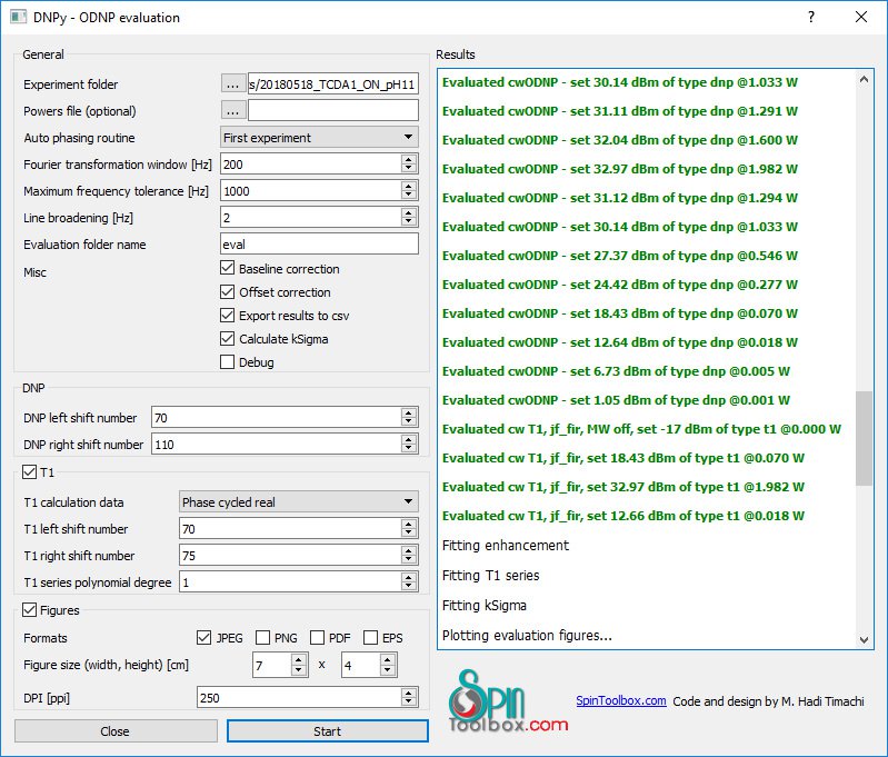
DNPyUI can be run with the following. It will show you an intuitive UI.

python3 DNPyUI.py

5.2 Function call

If you prefer to use DNPy as a function call, you can import functions and setup kwargs for return_exps() function. A sample usage is implemented in dnpEval.py. You need to set the following variables in your dnpEval:

path = '/path/to/exp/folder/'
powerFile = 'powers'
kwargs = {
    't1Calc': 'PCreal',  # 'PCreal' for real phase cycled channel or 'PCmagn' or 'real' or 'magn'
    'phase': 'first',  # all, none, first
    'ftWindow': 200,  # X domain for FT plot, int. and phase calculation
    'maxWin': 1000,  # Does not allow peaks out of this domain to be calculated in int.
    'lS': 70,  # Left shift points or 'auto'
    'lSt1': 70,  # LS for t1 experiments (this differs from DNP sometimes)
    'rS': 110,  # Right shift points
    'rSt1': 75,
    'lB': 2,  # Line boradening [Hz]
    'offCor': True,  # offset correctioon
    'basCor': True,  # baseline correction
    'evalPath': 'evalHadiTest',
    'plotDpi': 250,  # plot file resolution
    'plotExts': [],  # remove all if you do not want plots to be saved
    'process': True,
    'debug': False,
    'dumpToCsv': True,
    'figSize': (13, 8),
    'powerFile': powerFile,
    't1SeriesEval': True,
    't1SeriesPolDeg': 1,  # Polynomial degree for T1 series fit (default = 1)
    'kSigmaCalc': True,
}

path defines the ODNP experiment root folder.
powerFile is used when you have "ODNP - set .. dB" style title in your experiments and is a csv file containing dB to dBm conversion table.
debug boolean turns verbose evaluation on and gives you more information.
plotExts denotes the plot file extensions you want to have saved.

Finally, we call the main function using:

exps = return_exps(path, **kwargs)

DNPy can be downloaded from the github page.

Created: 2018-06-07 Thu 09:44

Modified: 2018-07-02 Mon 15:56

Validate

Changelog

2018.06.29:

Added cross-OS user interface using PyQt platform
Fixed some unexpected errors

2018.06.07 initial release:

ODNP enhancement experiments evaluation
T1 calcuation and series fit
kSigma calculation with uncorrected and corrected model (in case there are T1 power series experiments)
Plot to all required file formats for each experiment along with collective results

Table of Contents